Introduction
Tensile test simulations provide a valuable means of verification and validation of material models before proceeding to more complex component level or system level simulations
2 examples are provided here for the characterization of steel material data for OpenRadiossusing Material Laws 2 and 36 with and without strain rate dependency and introduce the concept of triaxiality when considering failure.
...
| Expand | ||||||||||||||
|---|---|---|---|---|---|---|---|---|---|---|---|---|---|---|
| ||||||||||||||
IntroductionThe purpose of this example is to introduce a method for characterizing and validation of the most commonly used OpenRadioss material laws for modeling elasto-plastic materials. The use of "engineering” and "true” stress-strain curves is pointed out. Failure models are also introduced to better fit the experimental response. Input FilesModel Files: Section 1 (74 KB) Options and Keywords UsedKeyword documentation may be found in the reference guide available from OpenRadioss User Documentation
Model DescriptionTension is applied to an object. The standardized “dogbone" object contains a defined cross-sectional area A0, The material to be characterized is DP600 Steel. (Ref. 1) A velocity is imposed at the right-end. Units: mm, ms, kg, N, GPa. The material undergoes isotropic elasto-plastic behavior which can be reproduced by a Johnson-Cook (/MAT/LAW2). The tabulated material law (/MAT/LAW36) is also studied. The model is meshed with 4-node shells and 3-node shells as shown in Figure 2. The average element size is about 2 mm. The shell properties use recommended best practice settings, except for the thickness which matches the test.
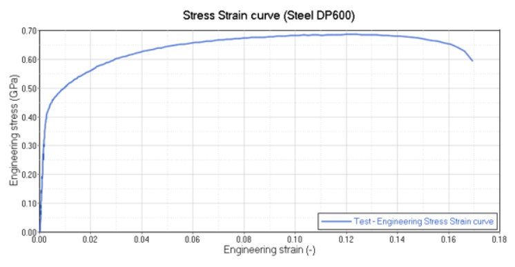
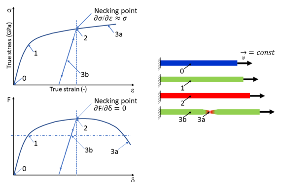
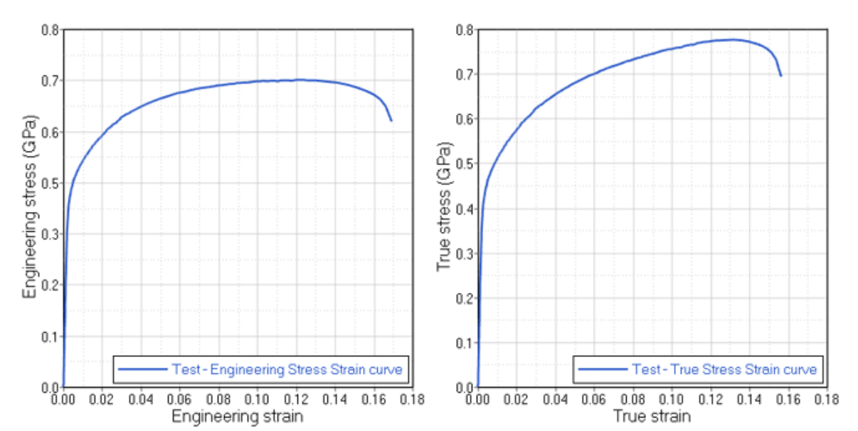
Boundary ConditionsThe left side of the object is fixed in all six degrees of freedom (all three translational and all three rotational DOFs). On the right side only translation in X-direction is free, all other five DOFs are fixed. An imposed velocity of -1.0 m/s in the X-direction is applied to the main node of the rigid body, shown Figure 2, whereby the elongation is increased uniformly at low speed. Two measurement nodes with a distance of 80 mm are chosen (Figure 3) to continuously measure the change in length Δl in the measurement section of the sample during the simulation and to obtain the strain εe on the sample. The engineering (nominal) stress is calculated as: (Equation 1) The total engineering strain is calculated as: (Equation 2) The true strain is computed with the relationship: (Equation 3) Engineering strain and true strain; therefore, are linked together by: (Equation 4) True stresses are measured by dividing the force with the true deformed section: (Equation 5) Thus, to compute true stresses, the area variation must be considered. If Poisson’s coefficient is 0.5 during plastic deformation, the true area in mono-axial traction is: (Equation 6) Thus, the relationship between true and engineering stresses is: (Equation 7) Characterization of the Material LawThere are two steps to characterize the material law. Transform the engineering stress versus engineering strain curve into a true stress versus true strain curve (this step applies to any elasto-plastic material law). Extract the main parameters from the true stress versus true strain curve, to define the material law (Johnson-Cook law and material coefficients for /MAT/LAW2 or the yield curve definition for /MAT/LAW36). When there is no material test data available (for example, in an early design stage), values of Yield stress, Ultimate tensile strength (engineering stress value) and Engineering strain at UTS must be provided to characterize /MAT/LAW2 using Iflag = 1. The characterization will be made for /MAT/LAW2 (Johnson-Cook elasto-plastic), and /MAT/LAW36 (tabulated elasto-plastic). For each of the material laws, the yield stress and Young's modulus are determined from the curve. The plastic strain can be defined as: (Equation 8) An important point to be characterized on the curve is the necking point, where the slope of the force versus the displacement curve is equal to 0, and where the following relationships apply: (Equation 9)
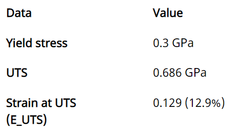
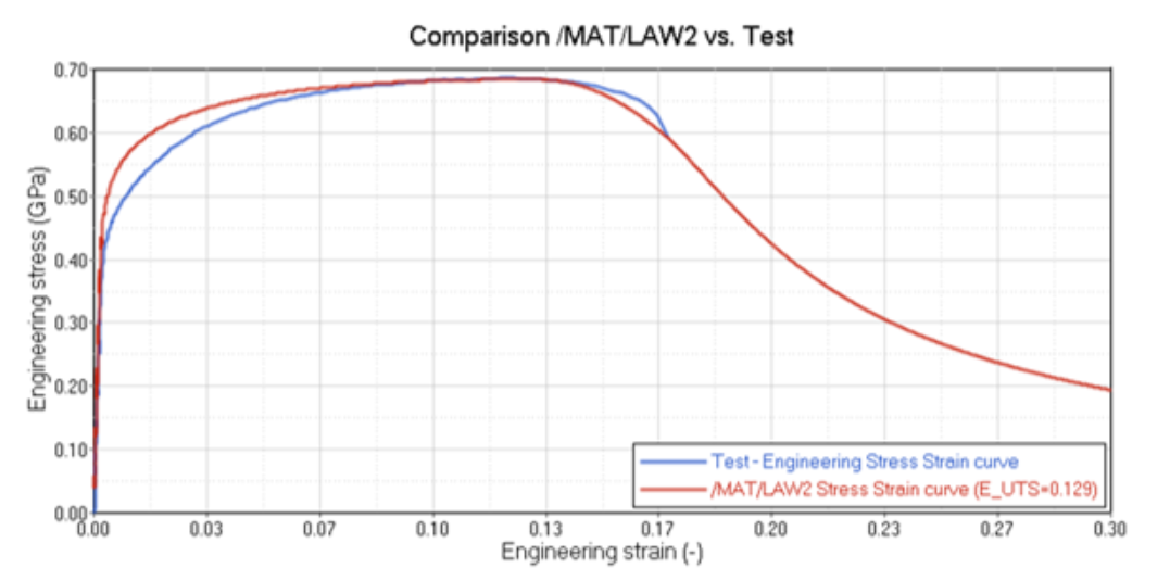
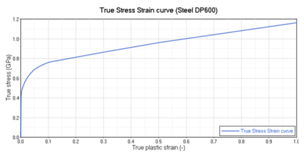
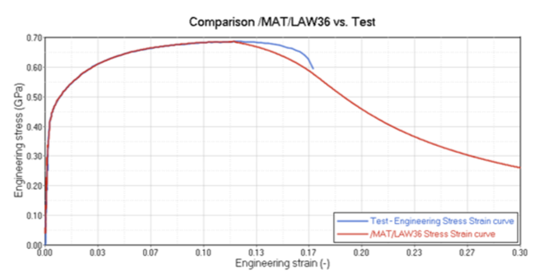
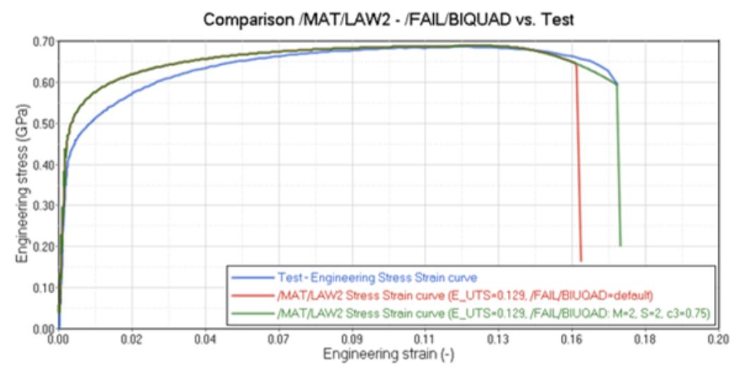
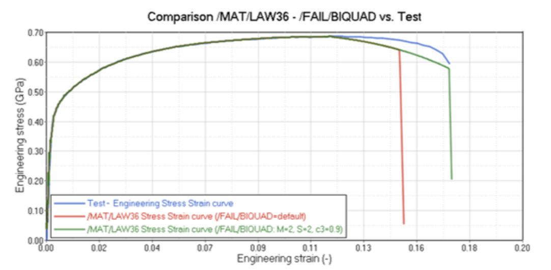
Results/MAT/LAW2: Elasto-plastic Material Law using the Johnson-Cook ModelThe stress versus plastic strain law is: (Equation 10) If the material parameters b and n are not available, then OpenRadioss can use /MAT/LAW2, Iflag = 1. In this case, the UTS (Ultimate tensile strength, engineering value) and engineering strain at UTS are entered. These values can often be found online, in literature or from a material supplier. OpenRadioss will then calculate the b and n parameters used in the Equation (Equation 10). Normally if a real test stress-strain curve exists, the test data should be used in /MAT/LAW36 (PLAS_TAB). However, in this example, you will assume that the test curve is not available and use /MAT/LAW2 with Iflag = 1 to see how well using the simplified data input compares to the actual test curve. Since the simulation calculates true stress and true strain for the elements, the engineering stress-strain curve from the simulation must be calculated. Similar to the test, the engineering stress can be calculated by using the Engineering nominal stress equation (Equation 1) and the rigid body force and original area. The engineering strain can be calculated by using total Engineering Strain equation (Equation 2) and the displacement between the two measurement nodes and the original distance. In the model, the displacement of node 616 is measure with respect to the displacement of node 102 by using a local moving system placed at node 102. This allows the displacement between the two nodes to be output as the displacement of node 616. Comparing the simulation results of the stress-strain curve show a perfect agreement with respect to the maximum stress value of the tested curve. The initial behavior of the simulation curve before the necking point shows differences to the test curve (Figure 6) and the stress value is slightly higher. This can be improved by using /MAT/LAW36 and inputting the stress-strain curve test data. /MAT/LAW36: Elasto-plastic Material Law using a Tabulated Input FunctionSince tensile test data is available, a more accurate method is to use that data in material LAW36. The first step is to take the test data and calculate the true stress versus true plastic strain curve by using Equation 4 and Equation 7. The necking point is where the slope of the engineering stress-strain curve becomes zero. All values after the necking point can not be used for creating the material curve for /MAT/LAW36 and can be removed from the data and disregarded. Values after the necking point must be extrapolated to a strain larger than failure for the material. The necking point occurs at the engineering strain at the ultimate tensile stress = 0.129. After this point, the curve was linearly extrapolated to 100% plastic strain as shown in Figure 8. Next, the true stress versus true plastic strain is calculated using Equation 8. Using the curve in Figure 8 as input in LAW36, the simulation results perfectly match the test curve between yield point and the necking point, as shown in Figure 9. The post necking behavior depends on the method used to extrapolate the true stress versus true plastic strain data after necking. /FAIL/BIQUAD: Simplified Nonlinear Strain-based Failure Criteria with Linear Damage AccumulationIn some elasto-plastic material models, a single plastic strain at failure can be input to model material failure. The element is deleted when the plastic strain reaches a user-defined value εpmax The main disadvantage of using this approach is the element is deleted when the plastic strain is reached no matter the stress state. There is no difference between failure in tension or compression. Metals usually show different strains at failure for the different states of stress. Especially in the case of compression, the failure strain is usually much higher than for tension. To overcome this limitation, /FAIL/BIQUAD is used instead of the simple maximum equivalent plastic strain that can be defined in the material input. With a few simple inputs, /FAIL/BIQUAD creates a nonlinear plastic strain at failure as a function of stress triaxality. /MAT/LAW2 with /FAIL/BIQUADWhen the default high strength steel (HSS) values (M_flag =2) included in /FAIL/BIQUAD are used, the simulation shows failure before the test. To better match the test, the /FAIL/BIQUAD uniaxial tension plastic strain at failure value (c3) is increased from 0.5 to 0.75. Figure 10 shows the results for both simulation cases. /MAT/LAW36 with /FAIL/BIQUADSimilar to the LAW2 simulation, the /FAIL/BIQUAD uniaxial tension plastic strain at failure value (c3) is increased from 0.5 to 0.9 so that the failure point in the simulation matches the test. ConclusionIn the first part of the example, a method was introduced to characterize and validate the most commonly used OpenRadioss material laws. The /MAT/LAW2 (PLAS_JOHNS) material was used with a few material parameters to represent the material. The /MAT/LAW36 (PLAS_TAB) material was used with experimental data of a tensile test for a more accurate simulation. The use of "engineering” and "true” stress-strain curves was pointed out. To describe the failure behavior in tension and compression a simplified nonlinear strain-based failure criterion with linear damage accumulation (/FAIL/BIQUAD) was used to better fit the experimental response. References1: https://www.ssab.com/ SSAB – a stronger, lighter, and more sustainable world | ||||||||||||||
| Expand | ||
|---|---|---|
| ||
IntroductionThe strain rate effect is considered, and the influence of strain rate filtering studied. The changes in the mechanical properties at different loading speeds are caused by the increasing speed of the flow stress. As the flow stress increases, the fracture elongation can increase or decrease depending on the material. This also changes the energy a component can absorb in the event of a fast load before failure. In this example, the material strain rate influence with and without filtering will be studied. Input FilesModel Files: Section 2 (39 KB) Options and Keywords UsedKeyword documentation may be found in the reference guide available from OpenRadioss User Documentation
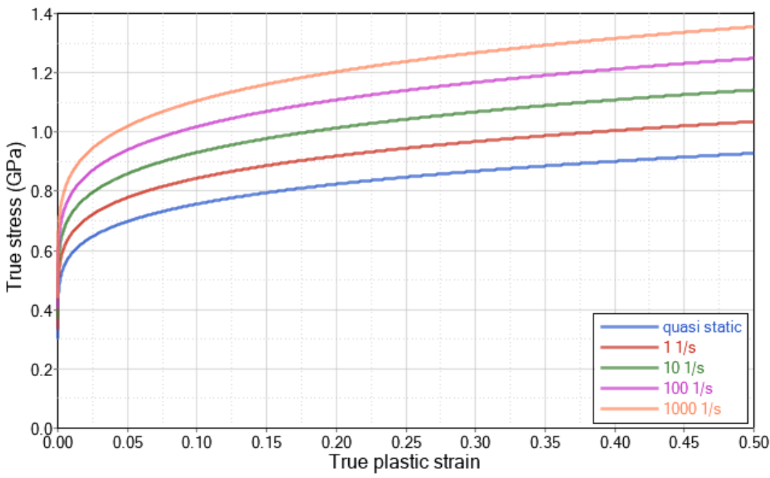
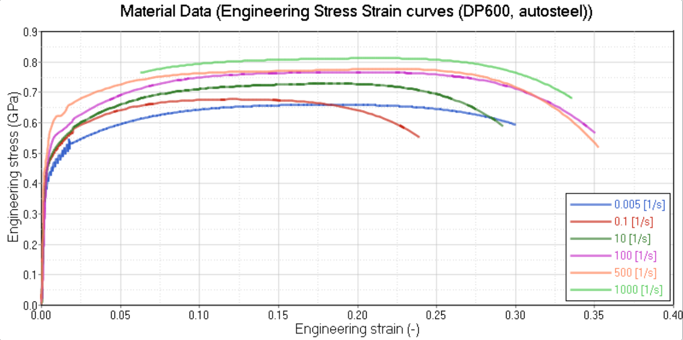
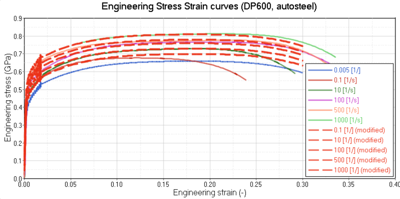
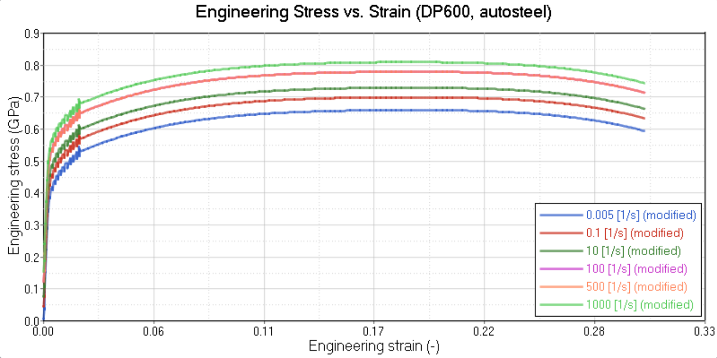
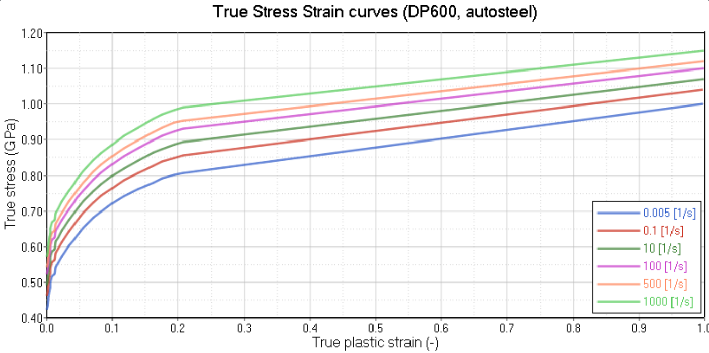
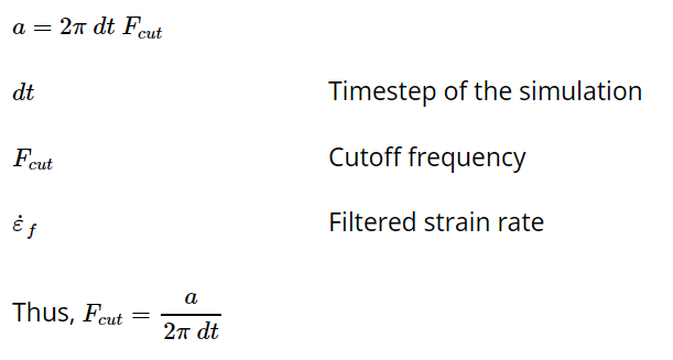
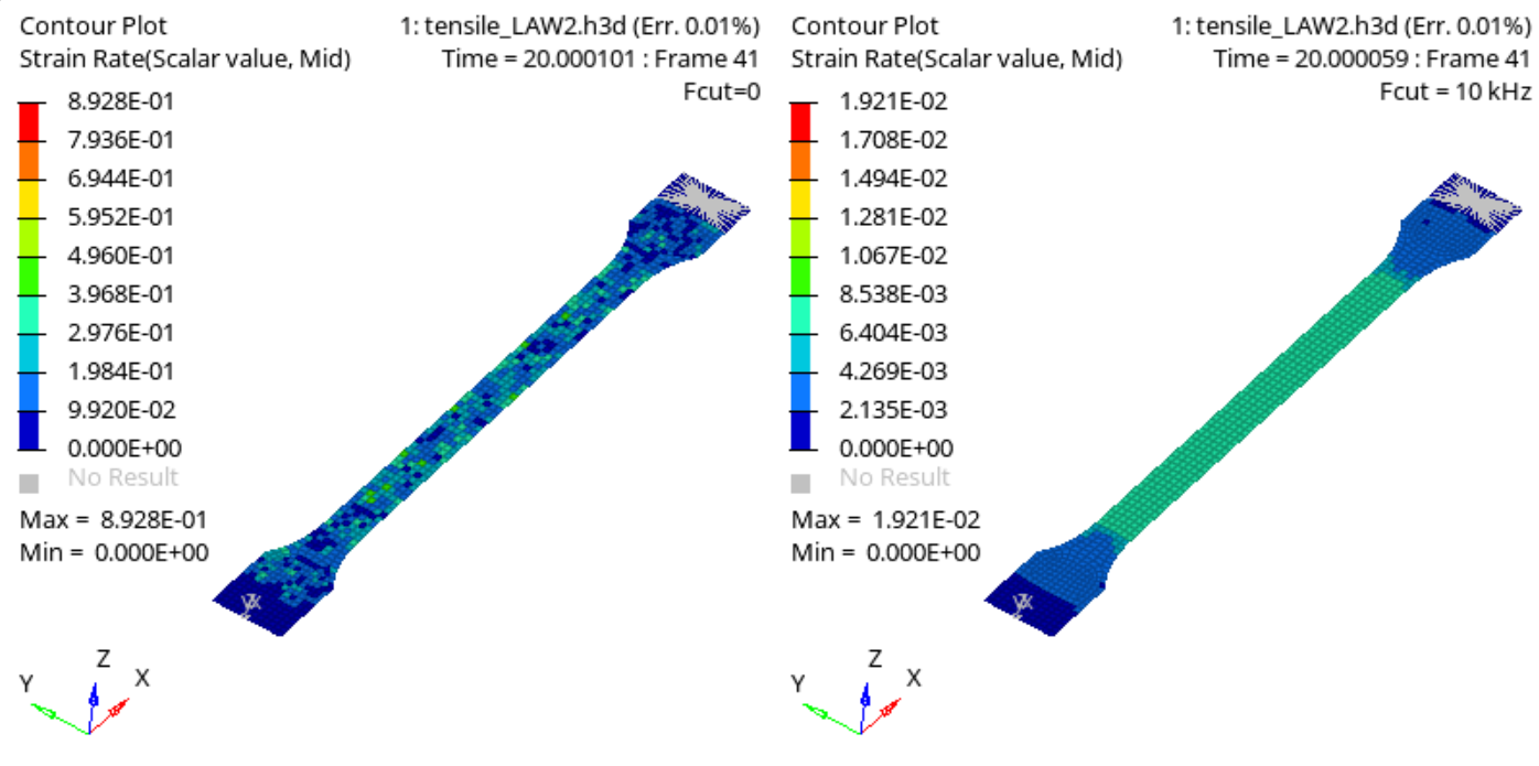
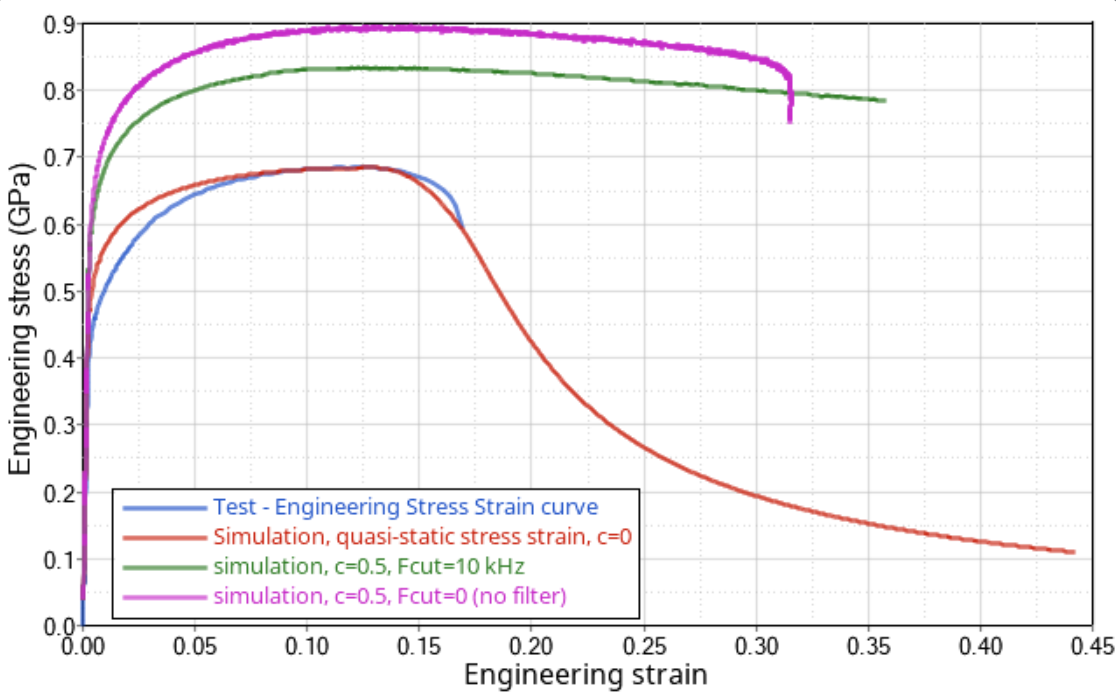
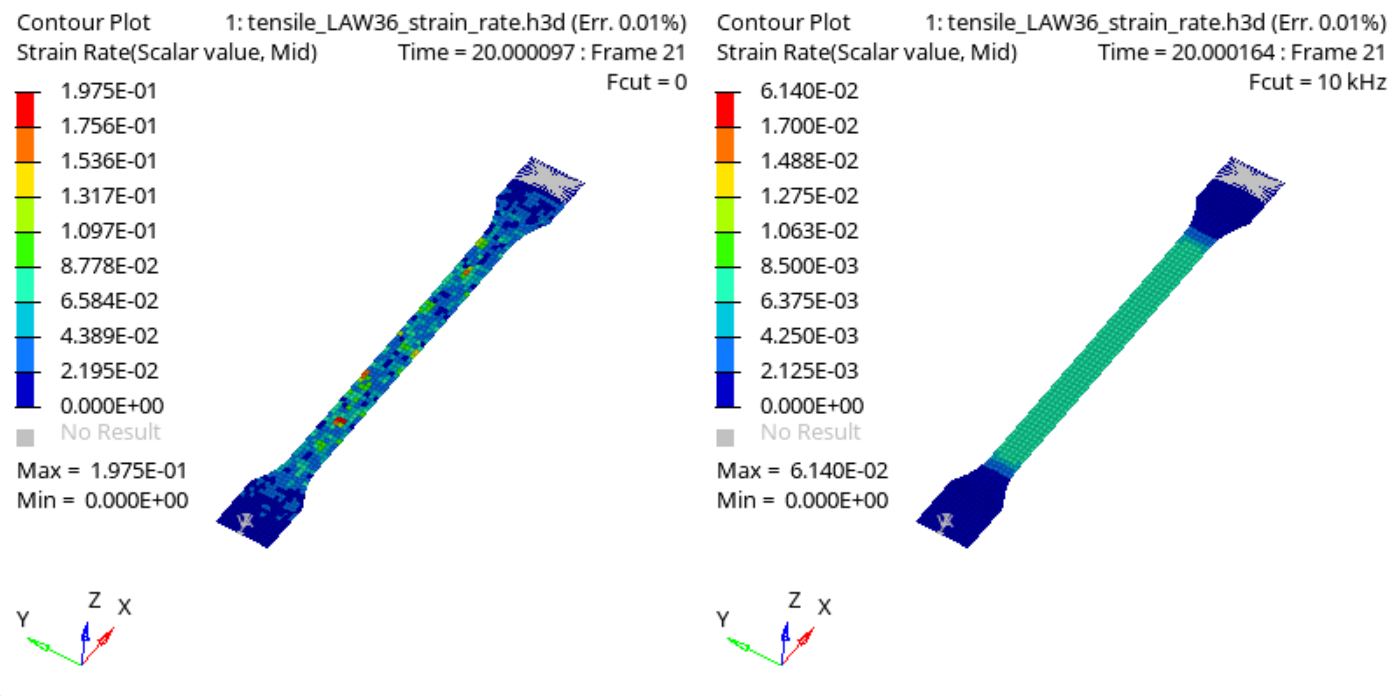
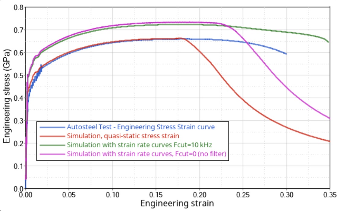
Model DescriptionIn Section 1, modeling a material’s elasto-plastic behavior based on one material test was looked at. For dynamic problems, the stiffness of a material can depend on the rate of deformation or strain rate. In this example, how to model the stiffness of the material as a function of the strain rate is outlined. First /MAT/LAW2 will be used with two coefficients that scale the stress strain curve depending on the strain rate. Next, test data at different strain rates is used with /MAT/LAW36 to model strain rate behavior of the material. The equivalent strain rate of each element is available as a contour output using the /ANIM/ELEM/EPSD or /H3D/ELEM/EPSD output request. The strain rate of a tensile test is calculated by dividing the velocity of the gauge region by the gauge length. In this model, the gauge length is measured from node 102 to node 616 and is 80 mm. The displacement and velocity of node 616 is output relative to a moving coordinate (/FRAME/MOV) attached to node 102. Thus, the displacement and velocity of the gauge length can be plotted directly from the relative displacement and velocity of node 616. Units: mm, ms, kg, N, GPa Since the time unit is ms, the strain rate unit used in the model is: /MAT/LAW2The Johnson-Cook plasticity model (/MAT/LAW2) is used to consider the strain rate effect on the elasto-plastic. The law reads as: (Equation 1) Where: The term scales the stress strain curve for strain rates that are greater than the reference strain rate. For strain rates less than the reference strain rate, there is no scaling. In this example, there is no test data, so approximate values of ε˙0 = 1x10⁻⁴ ms-1 and c = 0.05 are used to demonstrate the behavior. When the strain rate behavior of the material is not known, the strain rate coefficient is typically defined as c = 0 and; thus, there is no strain rate effect for the material. For further explanations about the Johnson-Cook model, refer to Elastic-plasticity of Isotropic Materials in the Radioss Theory Manual. /MAT/LAW36The second model uses the isotropic elasto-plastic material /MAT/LAW36 (PLAS_TAB) where user-defined stress versus plastic strain functions for different strain rates are derived from the real tests. 2 LAW36 will then use a linear interpolation between two different strain rate functions to calculate the material response for a particular strain rate. The input data for the material card is based on strain rate dependent test curves (Figure 2.) Due to high oscillation and other effects in the tested material (Figure 2), the curves must be modified in order to maintain numerical stability. In this example, the quasi-static curve was chosen as the initial curve and was shifted upwards until the best visual correlation to the other tested strain rate dependent curves was reached. This method avoids the intersections of different curves at higher strain rate regions (Figure 3 and Figure 4). The stress strain for each strain rate must not intersect. The true stress strain curves were derived from these new modified engineering stress strain curves. These curves were cut at the maximum stress and extrapolated to 100%. The same process described in Section 1 for LAW36 was used for each curve to create the following true stress versus plastic strain curves for use in /MAT/LAW36. ResultsBecause of the numerical application of the dynamic loadings, the strain rates are highly oscillating. This can lead to noisy results in the actual and local stress response. To obtain smooth and more physical stress results activate strain rate filtering by setting Fsmooth = 1 and defining a cutoff frequency using Fcut. The strain rate is filtered using an exponential moving average filter: (Equation 2) Where: The cutoff frequency is a function of the model timestep. Experience shows that the speed of the deformation is important also. For slower speeds like a car crash, 1 – 10 kHz (1000 – 10,000 Hz) is a good value, but for high-speed events, like ballistic, less filtering should be used, so 1 – 10 GHz is appropriate. Good engineering judgment should be used to determine a good value for each simulation. /MAT/LAW2 with Strain Rate EffectStarting with the LAW2 material input from Section 1, strain rate input was defined ε˙0 = 1x10⁻⁴ ms-1 and c = 0.05 to demonstrate the functionality (Figure 6 and Figure 7). The explicit scheme is an element-by-element method and the local treatment of temporal oscillations puts spatial oscillations into the model. A more physical strain rate distribution is achieved by filtering. Moreover, such results show oscillations in the stress strain curve when not damped by filtering. The strain rate of the entire tensile test can be calculated by dividing the velocity of the gauge length (velocity of node 616) by the gauge length (80 mm) which results in a strain rate, which ranges from 0.0075 ms-1 at the start of the simulation to 0.01 ms-1 at the end of the simulation. This corresponds well with the strain rate contour plot with strain rate filtering. Since the simulation strain rate speed is larger than the reference strain rate, ε˙0 = 1x10⁻⁴ ms-1 the material response is stiffer (Figure 7). /MAT/LAW36 with Strain Rate EffectSimilar to /MAT/LAW2, the results are smoothed when the strain rate filter is used (Figure 8). Similar to LAW2, the strain rate contour plot is similar to the strain rate calculated from the gauge length of the tensile test. As shown in Figure 9, a strain rate larger than the quasi-static test causes the material to be stiffer. The quasi-static and case without a filter, experience material necking which results in the reduction in stress. ConclusionStrain rate effects are important in dynamic events. LAW2 includes 2 parameters that can be used to add strain rate effects to the model. LAW36 allows separate stress versus plastic strain functions to be defined for different strain rates. No matter which material model is used, it is important to use strain rate filtering to reduce numerical noise and smooth the response. References1 SSAB – a stronger, lighter, and more sustainable world 2 The Voice of the American Steel Industry | American Iron and Steel Institute |
...


