Introduction
Impacts of rotating structures usually happen while the structure is rotating at a steady state. When the structure is rotating at very high speeds, it is necessary to include the centrifugal force field acting on the structure to correctly account for the initial stresses in the structure due to rotation.
Stage 1: shows how to use the /LOAD/CENTRI option in OpenRadioss to create the centrifugal force field and then apply an initial and imposed velocity to the rotating fan blades to correctly initialize the steady state rotating condition.
Stage 2: the rotating fan blades from Stage 1 are then impacted by a large hailstone/ice ball modeled using SPH particles. To correctly model the failure of the blades, a OpenRadioss material failure model is applied to them.
...
Figure 1.
Stage 1: Fan Blade Rotation Initialization
The /LOAD/CENTRI option in OpenRadioss is used to create the centrifugal force field on fan blades.
Input Files Stage 1
| Expand | |||||||||||||||||||||||||
|---|---|---|---|---|---|---|---|---|---|---|---|---|---|---|---|---|---|---|---|---|---|---|---|---|---|
| |||||||||||||||||||||||||
Fan Blade Rotation InitializationThe /LOAD/CENTRI option in OpenRadioss is used to create the centrifugal force field on fan blades. In a second Engine file an initial velocity is applied to the model and a /SENSOR is used to deactivate the /LOAD/CENTRI force and apply an imposed velocity to the blades center of rotation. Options and Keywords UsedKeyword documentation may be found in the reference guide available from OpenRadioss User Documentation
When the second Engine file starts, an initial and constant imposed rotational velocity of 104.72 [rads] is applied to the blades. The imposed velocity (/IMPVEL) is activated using a time activated sensor (/SENSOR/TIME) at t=0.1 seconds. A sensor TYPE=NOT (/SENSOR/NOT) is used to turn off the centrifugal force when the imposed velocity is turned on. The /SENSOR/NOT activation state is opposite of the sensor it references and; thus, it will be on from time = 0 – 0.1 seconds. 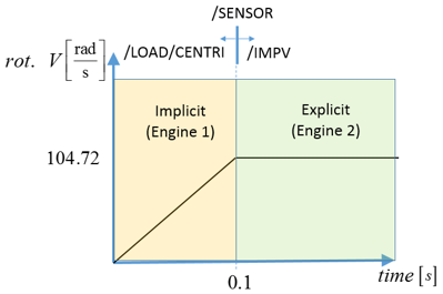 To keep the implicit solution in static equilibrium, a fully-constrained boundary condition (/BCS) is used on the main node of the rigid body that connects the base nodes of the blades. This fully-constrained boundary condition is removed in a second Engine file when rotation begins. Engine File 1: To activate the implicit solution, the following options are used.
Engine File 2: The initial rotational velocity is applied to the blade using the Engine option /INIV/AXIS/Z/1 and the z rotational boundary condition is released using /BCSR/ROT/Z to allow the blades to rotate.
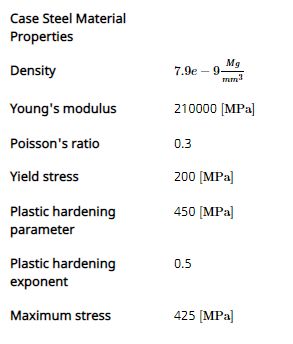
Model DescriptionFour fan blades are rotating at a steady state condition at 1000 RPM inside a simplified case. The base of each blade is attached to a rigid body which is constrained in all directions except rotation about the z axis. The stress in the blades caused by the steady-state rotation needs to be correctly modeled before other loads can be applied to the blades. The blades are assumed to be made of titanium with a constant 5mm thickness. The case is made of steel with varying thickness.  Units: mm, s, Mg, N, and MPa /MAT/PLAS_JOHNS, isotropic elasto-plastic material using the Johnson-Cook material model (see ref 1: Titanium properties) 
Boundary conditions:
Model MethodThe purpose of the analysis is to initialize the centrifugal force field and stress on the blades from a 1000 RPM rotation. One method to initialize the centrifugal force would be to slowly increase to rotational speed from 0 to 1000 RPM. However, for explicit simulations this can be very time consuming. To reduce the simulation time, the implicit solution method and the /LOAD/CENTRI option in OpenRadioss can be used to create the centrifugal force field. Using a second Engine file, an initial rotational velocity is applied to the blades and a /SENSOR is used to turn off the centrifugal force field and turn on an imposed velocity, (/IMPVEL). Now that the blades are rotating, the stress remains constant which means the blades are in steady-state rotation. ResultsIn Figure 3, the contour plot of the left side show the stress after applying the centrifugal force using /LOAD/CENTRI. The contour plot on the right shows that after 0.1 seconds of rotation at 1000 RPM the stress is still the same and thus, the blade is in a steady-state rotation condition. This demonstrates that the correct pre-load is applied.  Figure 4 demonstrates that the stress in the elements remains constant from 0.1 – 0.2 seconds during the steady-state rotation. This shows that the /LOAD/CENTRI creates the correct centrifugal force. 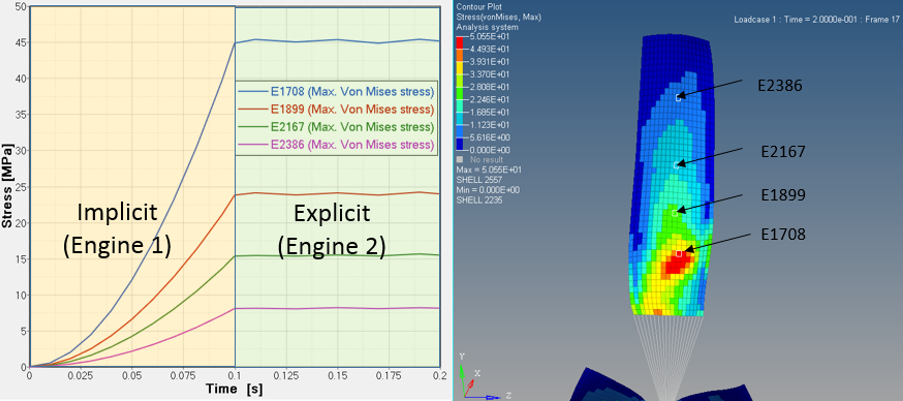 ConclusionNow that the force on the blades is correctly applied and the blades are rotating in a steady-state condition, a fan blade out simulation or blade impact by a bird or hailstone could be completed. See AlsoKeyword documentation may be found in the reference guide available from OpenRadioss User Documentation /FAIL/JOHNSON (Starter) /LOAD (Starter) /SENSOR (Starter) /INIV/AXIS/Keyword3 (Engine) References
|
Stage 2: Rotating Fan Blade Ice Impact and Failure
Two hailstone ice balls are added to the model from Stage 1: Fan Blade Rotation Initialization to study the deformation and failure of the blades when impacted.
Input Files Stage 2
| Expand | ||
|---|---|---|
| ||
Rotating Fan Blade Ice Impact and FailureTwo hailstone ice balls are added to the model from Stage 1: Fan Blade Rotation Initialization to study the deformation and failure of the blades when impacted. The stress in the blades, due to rotation is accounted for by using OpenRadioss state files, /STATE. A Johnson-Cook Failure model, /FAIL/JOHNSON, is applied to the blade elements to take into account material failure. Options and Keywords UsedKeyword documentation may be found in the reference guide available from OpenRadioss User Documentation
The stress state caused by the rotating blades, can be saved to a OpenRadioss State file, RUNAME_0001.sta, (/STATE/* keywords) and then applied to future analysis. This saves having to rerun the Radioss implicit pre-load step every time a design change would be made to the rest of the structure. The *.sta file contains the deformed nodal coordinates, elements definition, and initial stress state for the shell elements requested. Note: To make it easier to include the State file into the impact analysis, the nodes and elements of the parts in the State file are put into an include file, blade_nodes_elements.inc in Stage 1. Now to use the stress State file directly in a second analysis, replace the blade_nodes_elements.inc file by the State file (*.sta) from the implicit pre-load simulation. To create the State file, add the following commands to the end of the pre-load step from the first Engine file from Stage 1. and run the implicit pre-load simulation.
Now the hailstone ice ball model and the stress State file from the implicit simulation are included in the full simulation. The initial rotational velocity on the blades is included in the Engine file (/INIV/AXIS/Z/1) but could have also been be added Starter file using /INIVEL/AXIS. The ice impact simulation is ran for 0.08 seconds. Model DescriptionFour fan blades are rotating at 1000 RPM in a steady state condition inside a simplified case. The base of each blade is attached to a rigid body which is constrained in all directions except rotation about the z axis. The rotating blades impact two 3.07 kg hailstone ice balls which cause the blades to fail and then impact the case. The blades are assumed to be made of titanium with a constant 5mm thickness. The case is made of steel with varying thickness. 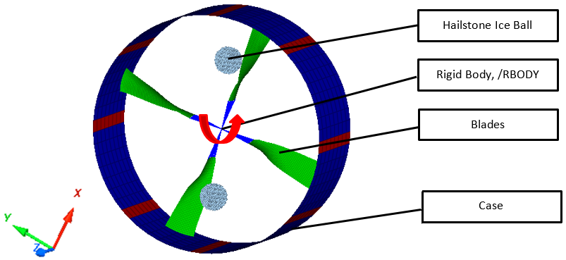 Units: mm, s, Mg, N, and MPa /MAT/PLAS_JOHNS, isotropic elasto-plastic material using the Johnson-Cook material model and Johnson-Cook failure model. (see ref 1: Titanium properties) 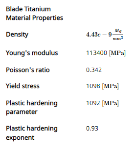 /FAIL/JOHNSON, Johnson-Cook ductile failure material. 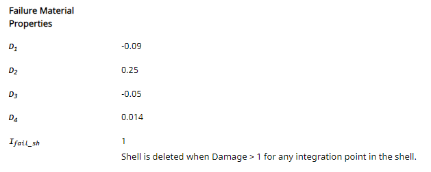
/MAT/HYD_JCOOK, isotropic elasto-plastic material using the Hydrodynamic Johnson-Cook material. 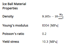 /EOS/POLYNOMIAL, a polynomial equation of state. 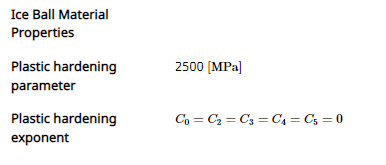 Boundary conditions:
Model MethodThis simulation builds on the results in Stage 1. The blades are impacted by two 3.07 kg hailstone ice balls with a radius of ~ 85 mm. A Johnson-Cook Failure model is added to the blade material to demonstrate how material failure can be modeled. The Johnson-Cook failure model relates plastic failure strain as a function of stress triaxiality (normalized mean stress). Additional details can be found in Materials of the Radioss User Guide, /FAIL/JOHNSON and /FAIL/TAB1. ResultsFigure 2, shows the blade stress at t=0.0 and that the initial pre-load stress in the state file was correctly included in the simulation. 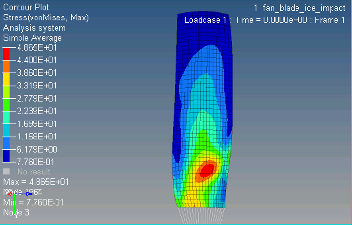 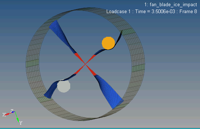 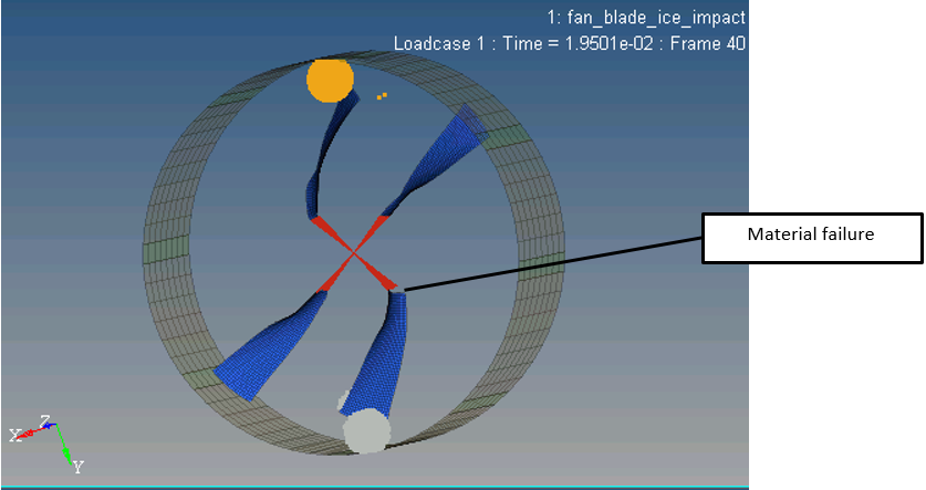 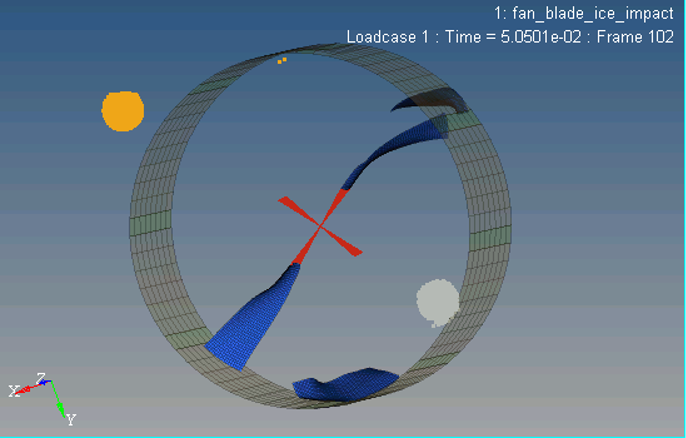 ConclusionThe stress in the blades from steady state rotation can be correctly accounted by including stress state files from a separate simulation. This saves time since it is not necessary to rerun the pre-load simulation for every design change of the case. The Johnson-Cook failure model accounts for the material failure of the blades due to their impact with hailstone ice balls. See AlsoKeyword documentation may be found in the reference guide available from OpenRadioss User Documentation /FAIL/JOHNSON (Starter) /FAIL/TAB1 (Starter) /LOAD (Starter) References
|